~2 meetings
A circuit simulator is a tool that helps engineers save resources such as time, material, and money, during the circuit development. It also helps to understand circuits better. There are a number of circuit simulators available on the market, some are free to use, while others cost way over 100,000 € for a yearly use. The differences between them can be a matter of discussion, but not now. At the beginning, you will probably discover the greatest difference between the simulators based on their "look". Although circuit simulators have been developed for almost as long as PCs have been around, they still look quite boring. Here is one example:
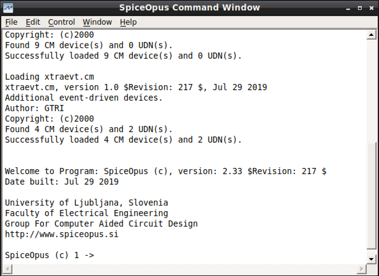
Oh no, it is a command-line tool. No schematic editor either.
Do not worry, you will get used to it. This is SpiceOpus, a SPICE (Simulation Program with Integrated Circuit Emphasis) based circuit simulator. Basically, SPICE is an equation solver, that relies on electronic component models and circuit description, which we call a netlist.
For installing the SpiceOpus, please follow these instructions (Windows, Linux, MacOS (Intel, M1)).
After successful installation, I invite you to create a folder with name lab_00 on your PC. Inside it, create an empty text file ex_00.cir. Let us write:
* My first circuit description
* This is a simple resistor with a voltage source.
v1 (1 0) dc=5
r1 (1 0) r=2k

.end
Let us have a look. The very first line is a name of a circuit. This line never gets interpreted, so you can also write it without the comment starting symbol *. Comments can only exist as a standalone line.
The netlist describes a simple circuit, consisting of only a voltage source v1, which we connected to nodes 1 and 0, and a resistor r1, which is connected in parallel to the voltage source v1, e.g., 1 and 0. Note that the first character of the device name encodes the device type, e.g., v in v1 stands for voltage source and r in r1 stands for resistor. The type-encoding character must be followed by a number or more characters that encode the instance. Note that v1 offers DC voltage of 5 V, and r1 has 2 kΩ resistance.
You probably wonder, where did the 1 and 0 come from. Those are node names, that we just made-up. Well, half-true! The nodename 1 was made up (it could easily be 2 or node1 or somenode), but the global ground node is always named 0. If no 0 (GND) exists in your circuit, simulator will complain with most weird error messages you can imagine.
Note that every netlist file has to end with .end.
Let us simulate this simple circuitry. Let us open the SpiceOpus and find out in which directory the program points at (works at). Type cd to the command line, and press enter. The working directory will be returned.
SpiceOpus (c) 1 -> cd
current directory: /home/vaje
SpiceOpus (c) 2 ->
Your ex_00.cir probably resides in another folder. Copy your file location from the file browser and paste it to SpiceOpus command-line, followed after cd again:
SpiceOpus (c) 1 -> cd /media/sf_vbox_share_fold/CAO/CAO202223/LAB/lab_00
current directory: /home/vaje
SpiceOpus (c) 2 ->
In Windows, your path will look something like:
SpiceOpus (c) 1 -> cd "C:/Documents and Settings/All Users/Documents/CAO/CAO202223/LAB/lab_00"
Remember to change backslashes \ to normal slash / and add double dictation marks "" when the path includes empty spaces.
Now load your ex_00.cir file into the simulator:
SpiceOpus (c) 2 -> source ex_00.cir
SpiceOpus (c) 3 ->
No output means good output (means - no errors!). Now we can run our first circuit analysis, the "Operating Point" analysis, or shortly op:
SpiceOpus (c) 2 -> source ex_00.cir
SpiceOpus (c) 3 -> op
If any error messages were thrown, read them carefully and apply corrections. But normally, when no errors, you get no output. No output is good output. Now we can observe results. Let us type:
SpiceOpus (c) 3 -> print v(1)
This will tell you voltage between the nodes 1 and the ground.
SpiceOpus (c) 6 -> print v(1)
v(1) = 5.000000e+00
Interested in the current over the r1?
SpiceOpus (c) 12 -> print i(v1)
i(v1) = -2.50000e-03
SpiceOpus (c) 13 ->
Let us note that only current over a voltage source can be printed. When interested in some other branch current, you need to place a "dummy" voltage source (DC=0) and print current over it. There is a command that lists all available nodes and branch currents in your analysis:
SpiceOpus (c) 13 -> display
To be continued.
Pasting a file, created in our first session.

    * Butterworth Low-pass filter
    * more commentary

    v1 (in 0) dc=10 ac=1 sin=(0 10 1k  0  0)

    rs (in 1) r=2k
    c1 (1 0) c=0.8n
    c2 (out 0) c=0.8n
    l1 (1 out) l=6.4m
    rl (out 0) r=2k


    .control
    * Operation point analysis - initial state calculation
    op
    print v(in)
    print v(out)
    print v(1)
    * checking out currents:
    print i(v1)
    print i(l1)
    * type:
    * display
    * to see all results
    **************************************************************

    * SWEEP Analysis (DC Analysis)
    * Let us sweep the input voltage from 0-20V
    * dc source start stop step
    dc v1 0 20 0.1

    *plot v(out) xlabel "v(in)" ylabel "v(out)" title "Vi sweep"

    * We can also sweep a hardware parameter - e.g. resistance
    echo "Sweeping rl (load)"
    * at "rl"... sweep the parameter "r" from ... 1m ...19k with the step of 100

    dc @rl[r] 1m 10k 100
    *plot v(out)

    **************************************************************
    * AC Analysis
    * Create a BODE plot (frequency sweep)

    * got to your signal source and add ac=1
    ac dec 100 1 1meg

    * Firstly compute the transfer function
    let h=v(out)/v(in)
    let hmag=db(h)
    let hphase=unwrap(ph(h))

    *plot hmag
    *plot hphase

    **************************************************************
    * TRANSIENT (tran) ANALYSIS
    * Enable some time-dependent source

    *                       damping_factor_
    *                  delay_to_start____  \
    *             frequency[Hz]________  \  \
    *          half_amplitude_______   \  \  \
    *     signal_offset__________   \   \  \  \
    *                            \   \   \  \  \
    *vin1 (in inp)  dc=0 ac=1 sin=(0 0.05 1k  0  0)
    * OR do it inside a control block:
    * let @v1[sin]=(0;10;1k;0;0)

    * tran step stop start
    tran 1u 200m
    plot v(out) v(in)


    .endc


    .end